Session-4

Aim

• Learn about packages in R
• Use Bioconductor

Packages

Packages are collection of several functions in R.

To use a perticular function from a package, it need to be downloaded and loaded.

Install a package from CRAN

# download and install 'ggplot2' package from CRAN
install.packages("ggplot2")

Introduction to Bioconductor

Bioconductor is a collection of more than 1,500 packages for the statistical analysis and comprehension of high-throughput genomic data. Originally developed for microarrays, Bioconductor packages are now used in a wide range of analyses, including bulk and single-cell RNA-seq, ChIP seq, copy number analysis, microarray methylation and classic expression analysis, flow cytometry, and many other domains.

This session introduces the essential of Bioconductor package discovery, installation, and use.

Use Biocondutor

Discovering, installing, and learning how to use Bioconductor packages.

The web site at https://bioconductor.org contains descriptions of all Bioconductor packages, as well as essential reference material for all levels of user.

Install from Bioconductor

install.packages("BiocManager")
BiocManager::install(c("rtracklayer", "GenomicRanges"))

Application: RNASeq DGE Analysis

RNA sequencing (RNA-seq) has proven as a revolutionary tool since the time it has been introduced. The throughput, accuracy, and resolution of data produced with RNA-seq has been instrumental in the study of Transcriptomics in the last decade (Wang, Gerstein, and Snyder 2009). There are many applications of Transcriptomics data, today we going to discuss Differential Gene Expression (DGE) which is wildly used to study the expression pattern of genes in contrasting samples.

Most of the steps of RNA-seq analysis have become quite mature over the years, especially how to reach a read count table from raw fastq reads obtained from an Illumina sequencing run. We will demonstrate how to process the count table, make a case-control differential expression analysis, and do some downstream functional enrichment analysis.

About the data

For this exercise purpose we will be using the RNA-seq count table from a colorectal cancer study (SRA: SRP029880, collected from recount2 database), only protein coding genes were kept for the faster execution of the analysis.

Get to know the data

• RAW count data
• Metadata

Download the data

dir.create("data")
download.file(url = "https://github.com/bionivid-tech/r-workshop-sep-2020/raw/master/data/SRP029880.raw_counts.tsv", 
              destfile = "data/SRP029880.raw_counts.tsv")
download.file(url = "https://github.com/bionivid-tech/r-workshop-sep-2020/raw/master/data/SRP029880.colData.tsv",
              destfile = "data/SRP029880.colData.tsv")

Get data into R

Reading tabular in R.

counts <- read.table("data/SRP029880.raw_counts.tsv", sep = "\t", header = T, row.names = 1)
head(counts)

##          CASE_1 CASE_2 CASE_3 CASE_4 CASE_5 CTRL_1 CTRL_2 CTRL_3 CTRL_4 CTRL_5
## TSPAN6   776426 371725 612244 456147 513335 559544 489653 332084 238516 634115
## TNMD       1483    806   2995    297   1095   4631   1884   4484   1961   3976
## DPM1     364919 274342 248740 371045 325628 211173 123204 113606  67338 198331
## SCYL3    103601  97625  98387 117366 101943 160847 106890 106938  64928 101515
## C1ORF112  90805  59235  61460 108892  44839  52308  34236  38087  18522  58008
## FGR       57081 145623  26800 168519 158882  59723  24483  21608  18654  23682
##           width
## TSPAN6    12883
## TNMD      15084
## DPM1      23689
## SCYL3     44637
## C1ORF112 192074
## FGR       23214

metadata <- read.table("data/SRP029880.colData.tsv", sep = "\t", header = T, row.names = 1)
metadata

##                source_name group
## CASE_1 metastasized cancer  CASE
## CASE_2 metastasized cancer  CASE
## CASE_3 metastasized cancer  CASE
## CASE_4 metastasized cancer  CASE
## CASE_5 metastasized cancer  CASE
## CTRL_1        normal colon  CTRL
## CTRL_2        normal colon  CTRL
## CTRL_3        normal colon  CTRL
## CTRL_4        normal colon  CTRL
## CTRL_5        normal colon  CTRL

Normalization the data

In RNA-Seq, there are different type of normalization methods (such as - CPM, FPKM/RPKM, TPM) and some other method/package specific (Such as in DESeq2 - VST). Today we will calculate CPM and RPKM manually.

CPM

Counts per million (CPM) mapped reads are counts scaled by the number of fragments you sequenced (N) times one million. This unit is related to the FPKM without length normalization and a factor of 10^3 Ref

library(edgeR)
raw_counts <- subset(counts, select = c(-width))
cpm <- cpm.default(raw_counts)
head(cpm)

##               CASE_1     CASE_2      CASE_3      CASE_4     CASE_5     CTRL_1
## TSPAN6   133.0525426 69.0267115 118.0347011 63.45319990 75.1705899 83.6818109
## TNMD       0.2541349  0.1496685   0.5774069  0.04131475  0.1603471  0.6925826
## DPM1      62.5344859 50.9433750  47.9546579 51.61492360 47.6835767 31.5816791
## SCYL3     17.7536255 18.1282742  18.9680587 16.32642166 14.9280985 24.0552454
## C1ORF112  15.5608340 10.9995218  11.8488915 15.14762970  6.5660321  7.8228489
## FGR        9.7817077 27.0411643   5.1667799 23.44215745 23.2660030  8.9317887
##              CTRL_2     CTRL_3     CTRL_4      CTRL_5
## TSPAN6   90.8357832 63.7170750 66.1201154 116.5649088
## TNMD      0.3495018  0.8603467  0.5436178   0.7308802
## DPM1     22.8556382 21.7976235 18.6670761  36.4577954
## SCYL3    19.8292196 20.5182320 17.9989890  18.6607898
## C1ORF112  6.3511382  7.3077662  5.1345687  10.6632034
## FGR       4.5418541  4.1459346  5.1711610   4.3532958

RPKM

Reads per kilobase of exon per million reads mapped (RPKM), or the more generic FPKM (substitute reads with fragments) are essentially the same thing. Contrary to some misconceptions, FPKM is not 2 * RPKM if you have paired-end reads. FPKM == RPKM if you have single-end reads, and saying RPKM when you have paired-end reads is just weird, so don’t do it :). Ref

# create a vector of gene lengths 
geneLengths <- as.vector(subset(counts, select = c(width)))
# compute rpkm 
rpkm <- apply(X = subset(counts, select = c(-width)), 
                         MARGIN = 2, 
                         FUN = function(x) 10^9 * x / geneLengths / sum(as.numeric(x)))
options(scipen=999) # to off scientific notion of numbers
rpkm <- do.call(cbind, rpkm)
options(scipen=0, digits=7) # on again back
  
head(rpkm)

##                width       width      width       width      width      width
## TSPAN6   10.32776081 5.357968757 9.16205085 4.925343468 5.83486687 6.49552207
## TNMD      0.01684798 0.009922336 0.03827943 0.002738979 0.01063028 0.04591505
## DPM1      2.63981113 2.150507621 2.02434285 2.178856161 2.01289952 1.33317907
## SCYL3     0.39773339 0.406126625 0.42494027 0.365759833 0.33443328 0.53890820
## C1ORF112  0.08101479 0.057267105 0.06168920 0.078863509 0.03418491 0.04072831
## FGR       0.42137106 1.164864492 0.22257172 1.009828442 1.00224016 0.38475871
##               width      width      width      width
## TSPAN6   7.05082537 4.94582589 5.13235390 9.04796312
## TNMD     0.02317037 0.05703704 0.03603937 0.04845400
## DPM1     0.96482073 0.92015803 0.78800608 1.53901792
## SCYL3    0.44423280 0.45966871 0.40323026 0.41805654
## C1ORF112 0.03306610 0.03804662 0.02673224 0.05551612
## FGR      0.19565151 0.17859631 0.22276045 0.18752890

Quality check of samples

For quality check of samples we can do several studies such as PCA and Correlation.

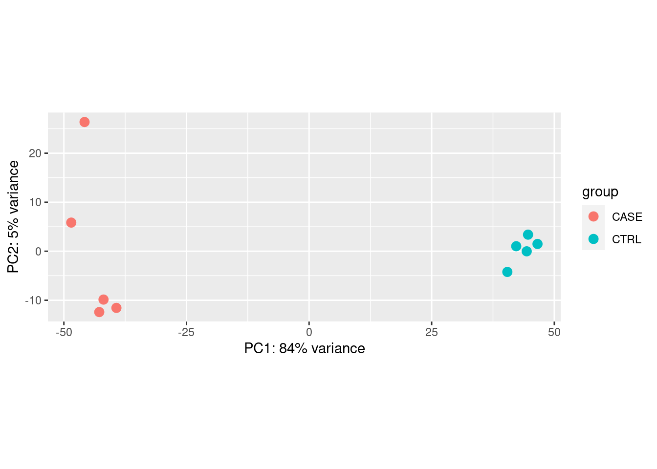
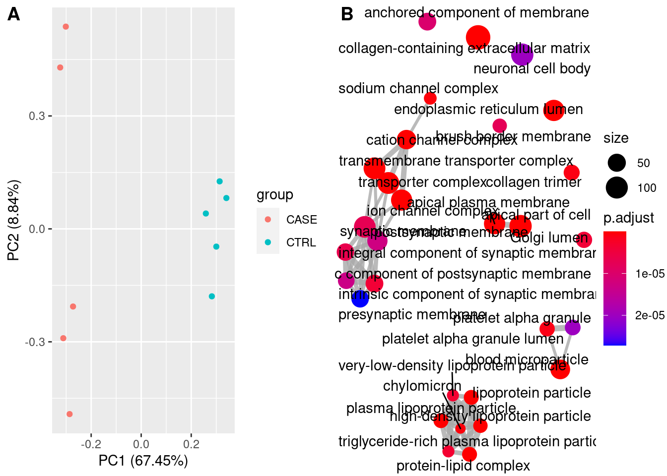
PCA

Principal Compound analysis on samples.

#transpose the matrix 
cpm_t <- t(cpm)
# transform the counts to log2 scale 
cpm_log <- log2(cpm_t + 1)
# calculate pca
pca <- prcomp(cpm_log)
summary(pca)

## Importance of components:
##                            PC1      PC2      PC3      PC4      PC5      PC6
## Standard deviation     80.0323 28.96809 23.83710 22.75690 18.86937 16.30932
## Proportion of Variance  0.6745  0.08837  0.05984  0.05453  0.03749  0.02801
## Cumulative Proportion   0.6745  0.76286  0.82270  0.87723  0.91473  0.94274
##                             PC7      PC8    PC9      PC10
## Standard deviation     15.39922 14.21772 10.223 1.039e-13
## Proportion of Variance  0.02497  0.02129  0.011 0.000e+00
## Cumulative Proportion   0.96771  0.98900  1.000 1.000e+00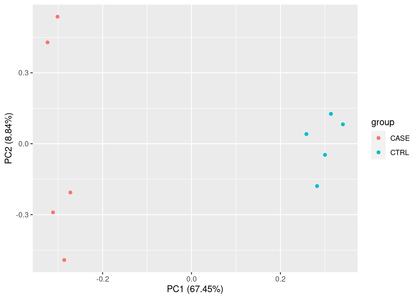

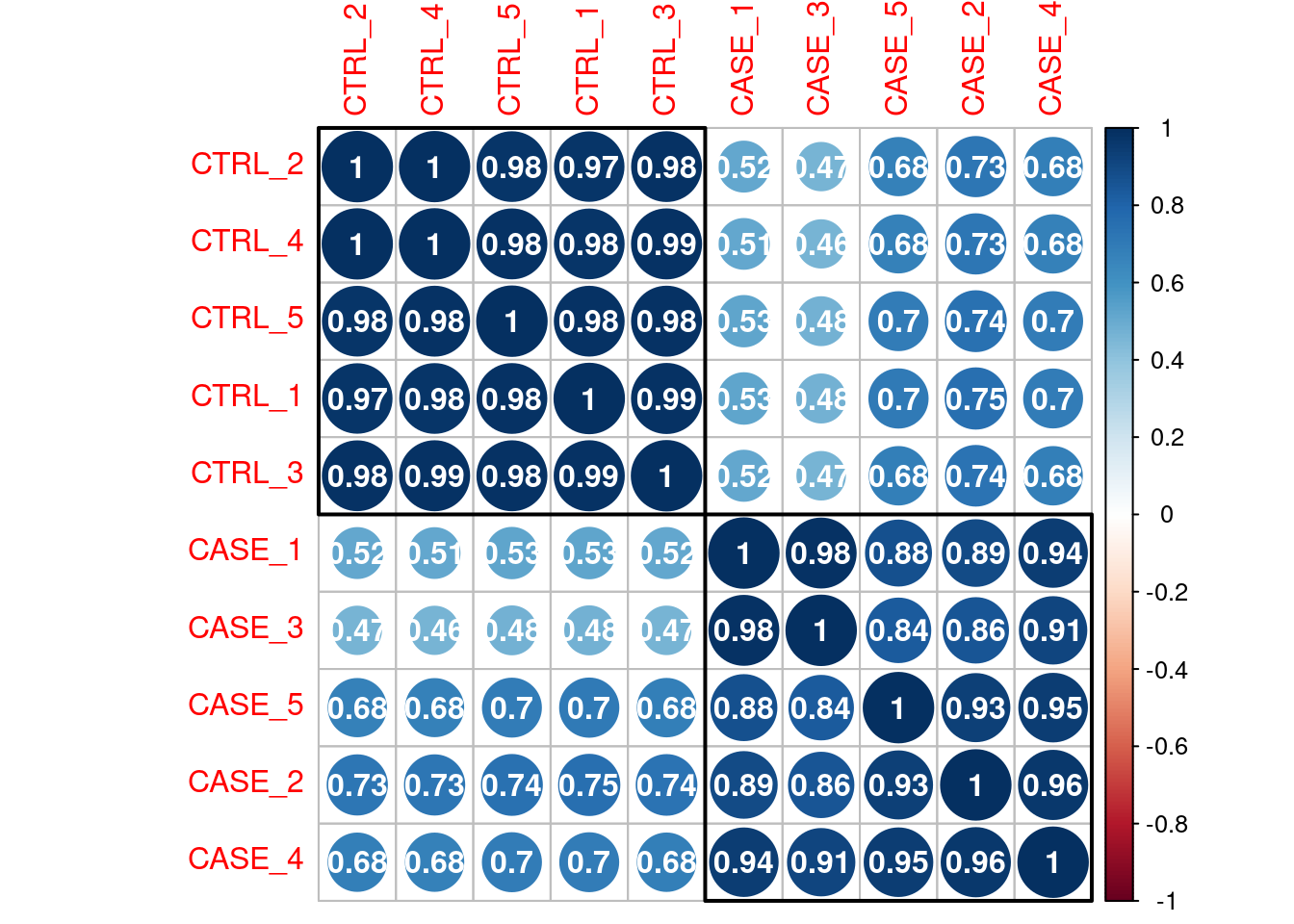
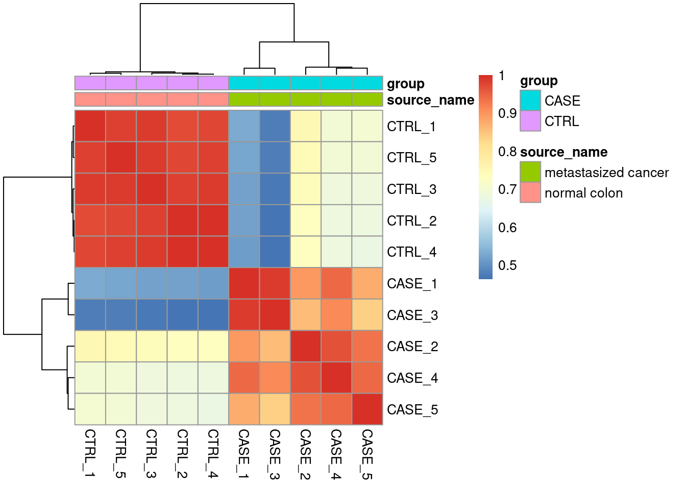
Plot PCA

Replicates should cluster together.

knitr::opts_chunk$set(echo = TRUE, warning=F, cache = F)

library(ggplot2)
library(ggfortify)
sample_pca <- autoplot(pca, data = metadata, colour = 'group')
sample_pca

Correlation

Sample to sample relation.

cor <- cor(cpm)
knitr::kable(cor)

	CASE_1	CASE_2	CASE_3	CASE_4	CASE_5	CTRL_1	CTRL_2	CTRL_3	CTRL_4	CTRL_5
CASE_1	1.0000000	0.8932785	0.9848753	0.9439505	0.8750504	0.5283715	0.5171387	0.5191767	0.5132126	0.5256384
CASE_2	0.8932785	1.0000000	0.8586247	0.9635875	0.9324452	0.7517934	0.7263228	0.7372209	0.7267303	0.7427978
CASE_3	0.9848753	0.8586247	1.0000000	0.9122808	0.8361842	0.4780616	0.4652480	0.4683691	0.4628397	0.4757110
CASE_4	0.9439505	0.9635875	0.9122808	1.0000000	0.9461943	0.6953668	0.6812613	0.6831496	0.6799802	0.6980752
CASE_5	0.8750504	0.9324452	0.8361842	0.9461943	1.0000000	0.7018531	0.6789861	0.6834173	0.6756385	0.6956374
CTRL_1	0.5283715	0.7517934	0.4780616	0.6953668	0.7018531	1.0000000	0.9712296	0.9886670	0.9784986	0.9803462
CTRL_2	0.5171387	0.7263228	0.4652480	0.6812613	0.6789861	0.9712296	1.0000000	0.9817525	0.9951188	0.9782734
CTRL_3	0.5191767	0.7372209	0.4683691	0.6831496	0.6834173	0.9886670	0.9817525	1.0000000	0.9871216	0.9849108
CTRL_4	0.5132126	0.7267303	0.4628397	0.6799802	0.6756385	0.9784986	0.9951188	0.9871216	1.0000000	0.9837302
CTRL_5	0.5256384	0.7427978	0.4757110	0.6980752	0.6956374	0.9803462	0.9782734	0.9849108	0.9837302	1.0000000

Correlation Plot

library(corrplot)
sample_cor <- corrplot(cor, order = 'hclust', addCoef.col = 'white', addrect = 2)

Sample heatmap

Sample heatmap with annotation

library(pheatmap)
sample_heatmap <- pheatmap(cor, annotation_col = metadata)

DEG Analsysis

Make the data ready.

#remove the 'width' column
countdata <- as.matrix(subset(counts, select = c(-width)))
head(countdata)

##          CASE_1 CASE_2 CASE_3 CASE_4 CASE_5 CTRL_1 CTRL_2 CTRL_3 CTRL_4 CTRL_5
## TSPAN6   776426 371725 612244 456147 513335 559544 489653 332084 238516 634115
## TNMD       1483    806   2995    297   1095   4631   1884   4484   1961   3976
## DPM1     364919 274342 248740 371045 325628 211173 123204 113606  67338 198331
## SCYL3    103601  97625  98387 117366 101943 160847 106890 106938  64928 101515
## C1ORF112  90805  59235  61460 108892  44839  52308  34236  38087  18522  58008
## FGR       57081 145623  26800 168519 158882  59723  24483  21608  18654  23682

metadata

##                source_name group
## CASE_1 metastasized cancer  CASE
## CASE_2 metastasized cancer  CASE
## CASE_3 metastasized cancer  CASE
## CASE_4 metastasized cancer  CASE
## CASE_5 metastasized cancer  CASE
## CTRL_1        normal colon  CTRL
## CTRL_2        normal colon  CTRL
## CTRL_3        normal colon  CTRL
## CTRL_4        normal colon  CTRL
## CTRL_5        normal colon  CTRL

Load the data into DESeq2 Object and design the experiment

library(DESeq2)
dds <- DESeqDataSetFromMatrix(countData = countdata, 
                              colData = metadata, 
                              design = ~ group) # experiment design
dds

## class: DESeqDataSet 
## dim: 19719 10 
## metadata(1): version
## assays(1): counts
## rownames(19719): TSPAN6 TNMD ... MYOCOS HSFX3
## rowData names(0):
## colnames(10): CASE_1 CASE_2 ... CTRL_4 CTRL_5
## colData names(2): source_name group

Remove genes with almost no information in any of the given samples.

#For each gene, we count the total number of reads for that gene in all samples 
#and remove those that don't have at least 1 read. 
dds <- dds[ rowSums(counts(dds)) > 1, ]

Run the analysis

dds <- DESeq(dds) # the only time taking step. 

## estimating size factors

## estimating dispersions

## gene-wise dispersion estimates

## mean-dispersion relationship

## final dispersion estimates

## fitting model and testing

dds

## class: DESeqDataSet 
## dim: 19097 10 
## metadata(1): version
## assays(4): counts mu H cooks
## rownames(19097): TSPAN6 TNMD ... MYOCOS HSFX3
## rowData names(22): baseMean baseVar ... deviance maxCooks
## colnames(10): CASE_1 CASE_2 ... CTRL_4 CTRL_5
## colData names(3): source_name group sizeFactor

Explore results

#compute the contrast for the 'group' variable where 'CTRL' samples are used as the control group. 
res = results(dds, contrast = c("group", 'CASE', 'CTRL'))
head(res)

## log2 fold change (MLE): group CASE vs CTRL 
## Wald test p-value: group CASE vs CTRL 
## DataFrame with 6 rows and 6 columns
##           baseMean log2FoldChange     lfcSE      stat      pvalue        padj
##          <numeric>      <numeric> <numeric> <numeric>   <numeric>   <numeric>
## TSPAN6   491987.63      0.0772416  0.283184  0.272761 7.85037e-01 8.68555e-01
## TNMD       2466.25     -1.4474155  0.631826 -2.290846 2.19723e-02 5.65051e-02
## DPM1     216809.25      0.9388739  0.200290  4.687581 2.76453e-06 2.28302e-05
## SCYL3    104400.07     -0.2843211  0.113732 -2.499919 1.24222e-02 3.54271e-02
## C1ORF112  53848.01      0.6299092  0.271324  2.321609 2.02540e-02 5.28672e-02
## FGR       63201.42      1.6468890  0.410016  4.016646 5.90324e-05 3.56989e-04

#sort results by increasing p-value
res <- res[order(res$pvalue),]
res

## log2 fold change (MLE): group CASE vs CTRL 
## Wald test p-value: group CASE vs CTRL 
## DataFrame with 19097 rows and 6 columns
##             baseMean log2FoldChange     lfcSE       stat       pvalue
##            <numeric>      <numeric> <numeric>  <numeric>    <numeric>
## CYP2E1       4829889        9.36024  0.215223    43.4909  0.00000e+00
## FCGBP       10349993       -7.57579  0.186433   -40.6355  0.00000e+00
## ASGR2         426422        8.01830  0.216207    37.0863 4.67898e-301
## GCKR          100183        7.82841  0.233376    33.5442 1.09479e-246
## APOA5         438054       10.20248  0.312503    32.6477 8.64906e-234
## ...              ...            ...       ...        ...          ...
## CCDC195      20.4981      -0.215607   2.89255 -0.0745386           NA
## SPEM3        23.6370     -22.154765   3.02785 -7.3170030           NA
## AC022167.5   21.8451      -2.056240   2.89545 -0.7101618           NA
## BX276092.9   29.9636       0.407326   2.89048  0.1409199           NA
## ETDC         22.5675      -1.795274   2.89421 -0.6202983           NA
##                    padj
##               <numeric>
## CYP2E1      0.00000e+00
## FCGBP       0.00000e+00
## ASGR2      2.87741e-297
## GCKR       5.04945e-243
## APOA5      3.19133e-230
## ...                 ...
## CCDC195              NA
## SPEM3                NA
## AC022167.5           NA
## BX276092.9           NA
## ETDC                 NA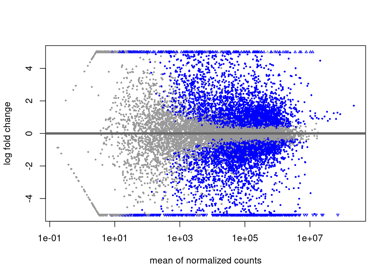

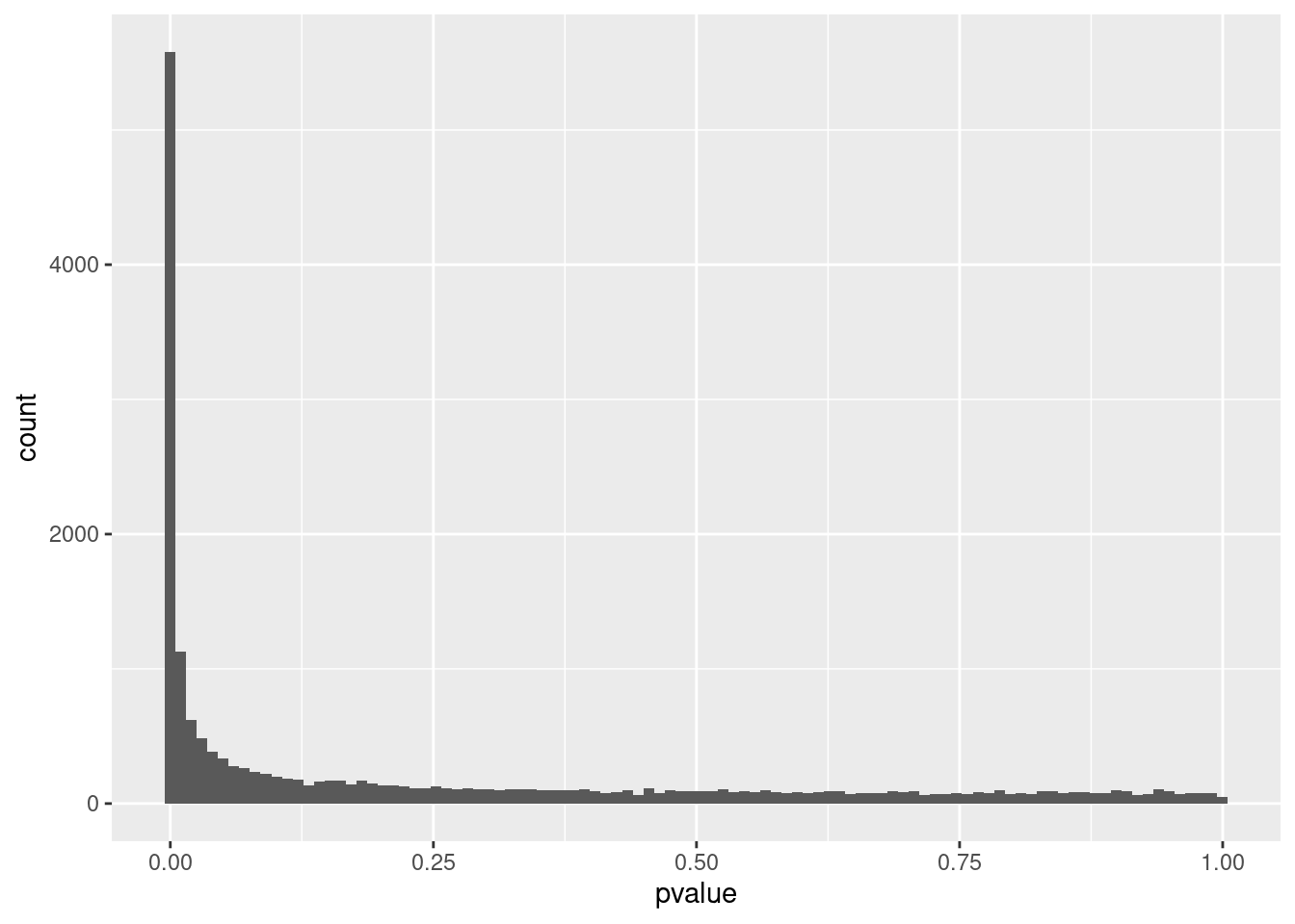
MA plot

DESeq2::plotMA(object = dds, ylim = c(-5, 5))

P-value distribution

ggplot(data = as.data.frame(res), aes(x = pvalue)) + geom_histogram(bins = 100)

PCA

For deseq normalized

rld <- rlog(dds)
plotPCA(rld, ntop = 500, intgroup = 'group')

Box plot

For deseq normalized

par(mfrow = c(1, 2))
boxplot(log(countdata), 
        col = as.numeric(as.factor(metadata$group)), 
        main = 'Raw Counts')
boxplot(log(counts(dds, normalized = TRUE)), 
        col = as.numeric(as.factor(metadata$group)), 
        main = 'Normalized Counts')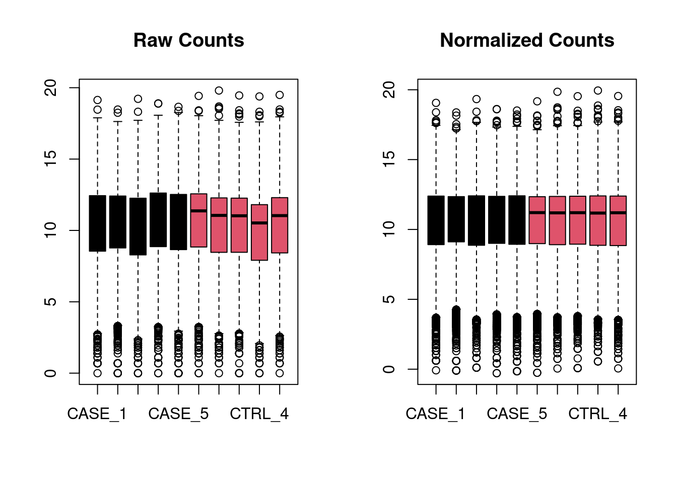

DGE Volcano plot

library(EnhancedVolcano)
EnhancedVolcano(res,
    lab = rownames(res),
    x = 'log2FoldChange',
    y = 'pvalue',
    title = "CASE vs CTRL",
    pCutoff = 0.05,
    FCcutoff = 2,
    pointSize = 3.0,
    labSize = 3.0)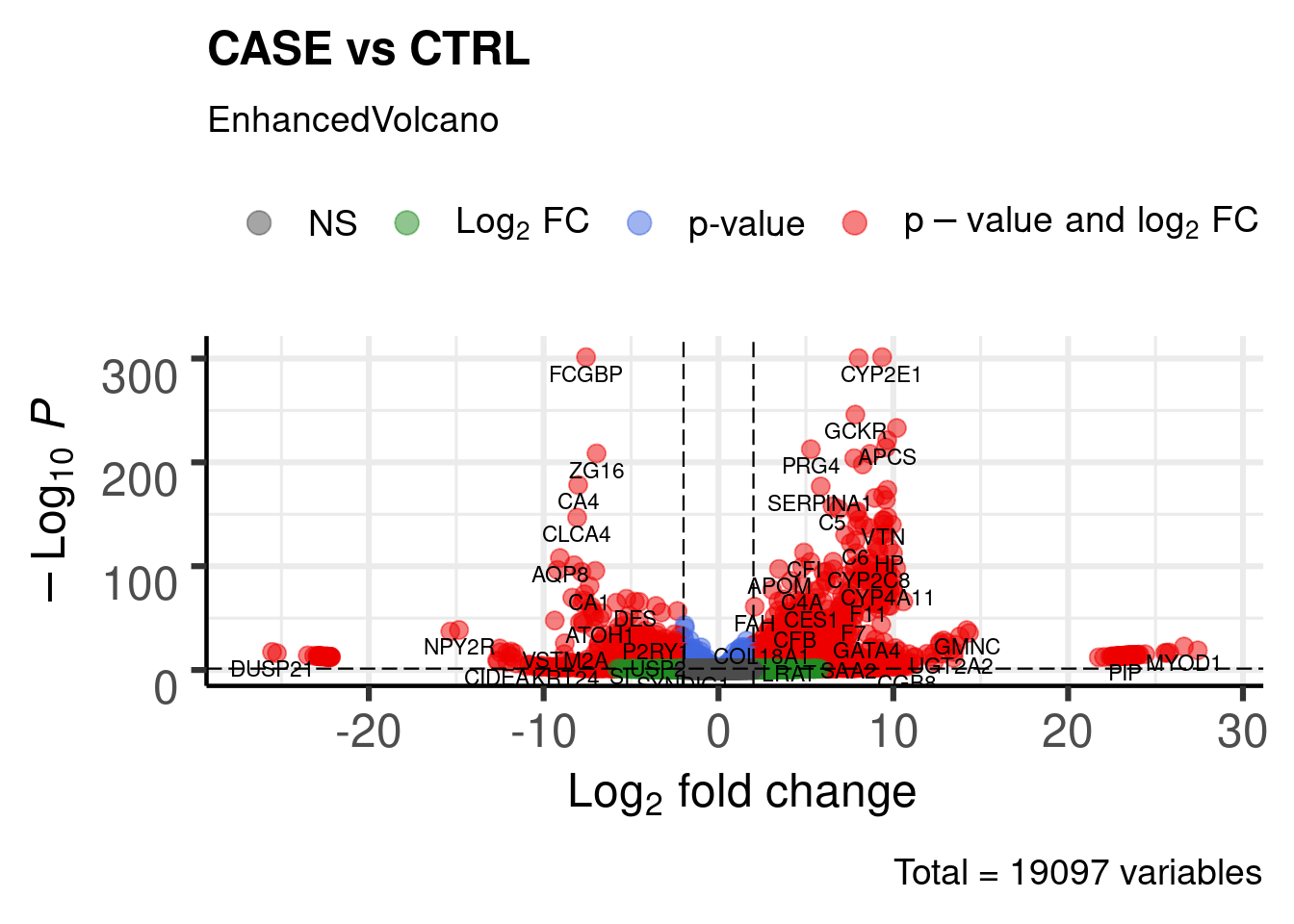

Extract results

Extract the DGE to make heatmap

library(dplyr)
library(tibble)
library(magrittr)
res_up <- res %>% as.data.frame() %>% 
  rownames_to_column('gene') %>%
  filter(log2FoldChange >= 2) %>% 
  mutate(reg_type = "Up regulation") %>% 
  column_to_rownames('gene')
head(res_up)

##         baseMean log2FoldChange     lfcSE     stat        pvalue          padj
## CYP2E1 4829888.9       9.360244 0.2152232 43.49088  0.000000e+00  0.000000e+00
## ASGR2   426421.7       8.018301 0.2162068 37.08626 4.678977e-301 2.877415e-297
## GCKR    100182.7       7.828413 0.2333762 33.54417 1.094790e-246 5.049446e-243
## APOA5   438054.0      10.202485 0.3125028 32.64766 8.649058e-234 3.191329e-230
## APCS    899875.4       9.649894 0.3033213 31.81410 4.131410e-222 1.270340e-218
## APOC4   152415.6       9.569025 0.3057277 31.29917 4.788978e-215 1.262169e-211
##             reg_type
## CYP2E1 Up regulation
## ASGR2  Up regulation
## GCKR   Up regulation
## APOA5  Up regulation
## APCS   Up regulation
## APOC4  Up regulation

res_down <- res %>% as.data.frame() %>% 
  rownames_to_column('gene') %>%
  filter(log2FoldChange <= -2) %>% 
  mutate(reg_type = "Down regulation") %>% 
  column_to_rownames('gene')
head(res_down)

##          baseMean log2FoldChange     lfcSE      stat        pvalue
## FCGBP  10349993.2      -7.575787 0.1864329 -40.63545  0.000000e+00
## ZG16    2122231.5      -6.974906 0.2258976 -30.87641 2.477314e-209
## CA4      842822.2      -8.025380 0.2813713 -28.52238 6.184050e-179
## CLCA4   1918679.3      -8.085007 0.3125788 -25.86550 1.628578e-147
## AQP8    1741004.4      -9.070041 0.4097381 -22.13619 1.417134e-108
## TMIGD1   325850.3      -8.257870 0.3857252 -21.40869 1.108936e-101
##                 padj        reg_type
## FCGBP   0.000000e+00 Down regulation
## ZG16   5.078219e-206 Down regulation
## CA4    8.776118e-176 Down regulation
## CLCA4  1.251901e-144 Down regulation
## AQP8   5.683630e-106 Down regulation
## TMIGD1  3.860143e-99 Down regulation

res_filt <- rbind(res_up, res_down)
# get up and down genes
res_filt_genes <- rownames(res_filt)
res_filt_genes[1:10]

##  [1] "CYP2E1" "ASGR2"  "GCKR"   "APOA5"  "APCS"   "APOC4"  "PRG4"   "ITIH3" 
##  [9] "A1BG"   "AADAC"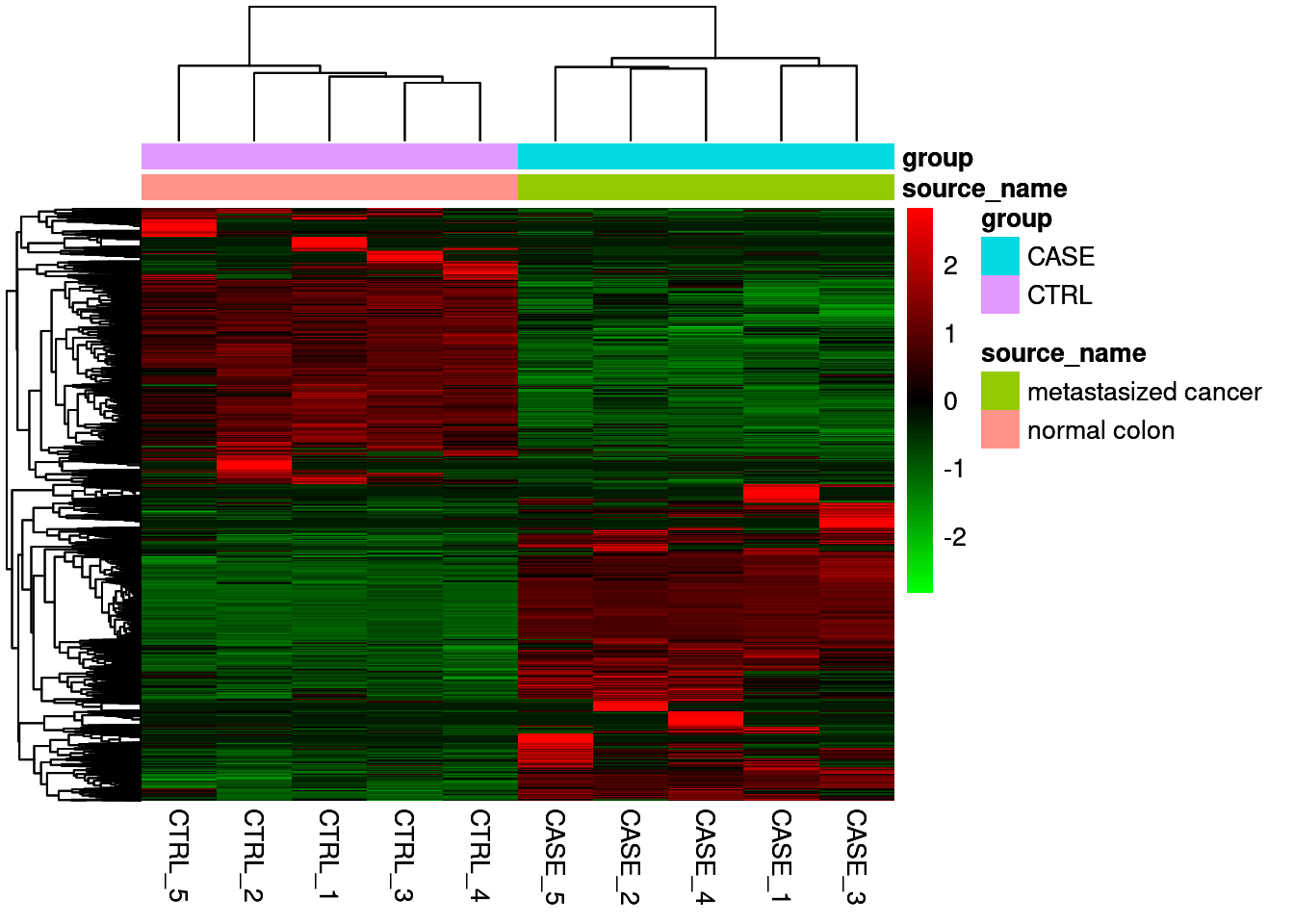

DGE Heatmap plot

vsd <- vst(dds)
vsd_count <- assay(vsd)
dge_heatmap <- pheatmap(vsd_count[res_filt_genes,],
                       col = gplots::greenred(75),
                       scale = "row",
                       show_rownames = FALSE , 
                       cluster_rows=TRUE, cluster_cols=TRUE, 
                       annotation_col= metadata)
dge_heatmap

Downstream analaysis

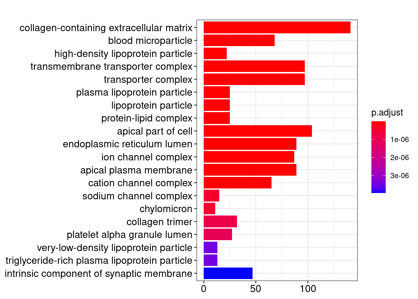
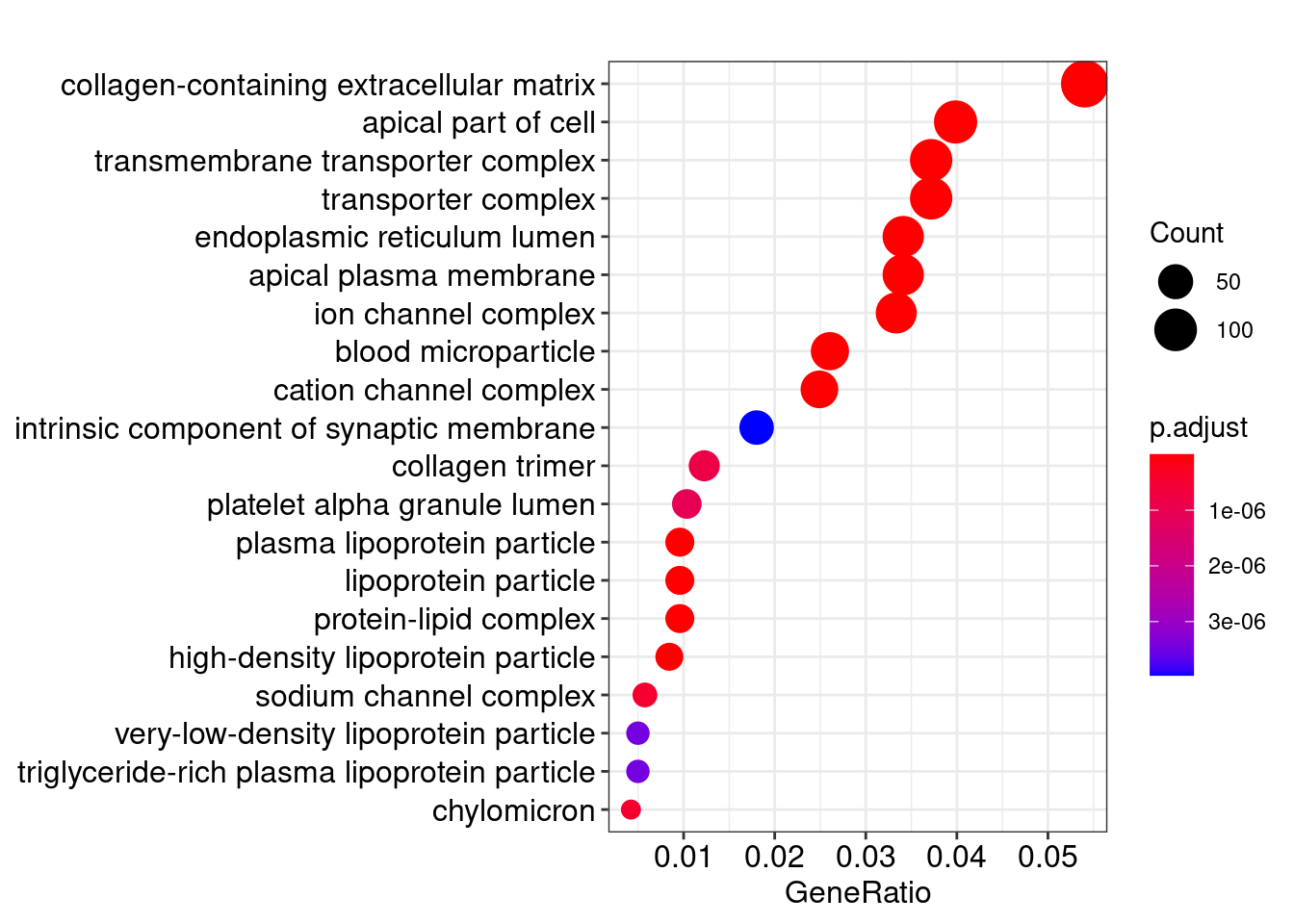
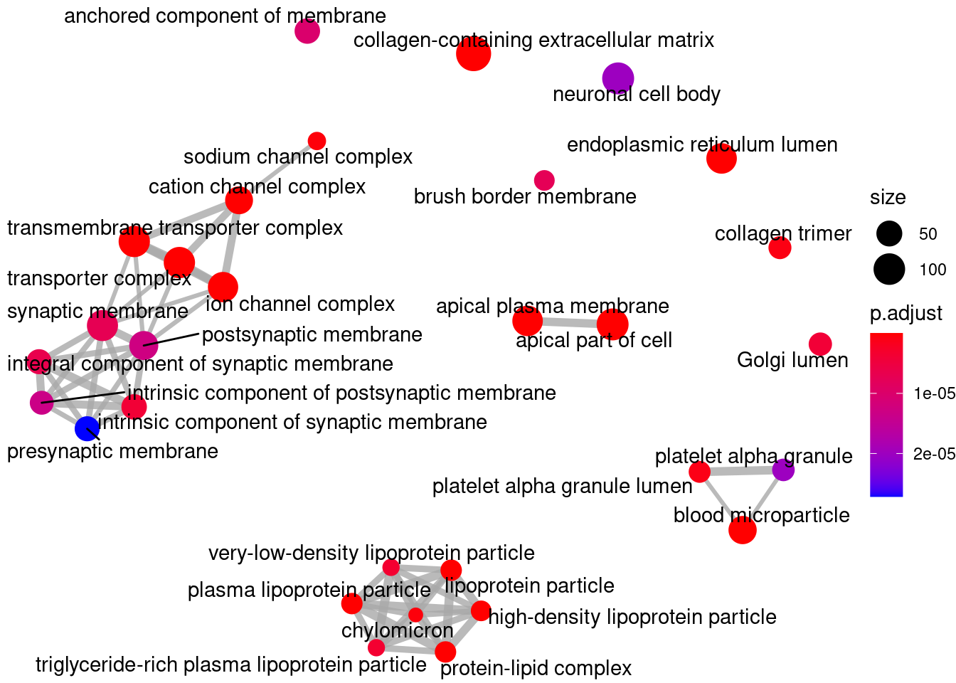
Gene Ontology

library(clusterProfiler)
library(org.Hs.eg.db)
ego <- enrichGO(gene          = res_filt_genes,
                OrgDb         = org.Hs.eg.db,
                keyType       = "SYMBOL",
                ont           = "CC",
                pvalueCutoff  = 0.01,
                qvalueCutoff  = 0.05)
knitr::kable(head(ego@result))

	ID	Description	GeneRatio	BgRatio	pvalue	p.adjust	qvalue	geneID	Count
GO:0062023	GO:0062023	collagen-containing extracellular matrix	141/2609	406/19717	0	0	0	APCS/PRG4/A1BG/SERPINA1/HPX/SERPINA5/ITIH4/VTN/APOC3/APOA1/ORM2/APOH/PLG/ITIH2/F2/SERPINA3/SERPINF2/ITIH1/F9/AMBP/FGA/ORM1/AHSG/FGG/SERPINC1/FGB/SERPING1/CDH2/F7/F12/FN1/AGT/MST1/INHBE/COL18A1/CLU/HRG/KNG1/ANG/PZP/ADAMTS2/THBS2/APOE/SERPINE1/MBL2/COL10A1/BGN/COL6A6/TGM2/SPP2/SMOC1/COL4A1/AZGP1/ASPN/CTHRC1/CFP/SDC2/USH2A/TIMP1/ANXA8/ADAMTS4/TGFB3/COL4A2/COL1A1/COL26A1/TGFBI/COMP/SULF1/APOA4/COL11A1/SEMA7A/COL25A1/MATN3/MMP9/VWA2/MMP8/DEFA1/BMP7/CBLN4/WNT2/PRTN3/LAMB4/SOST/WNT8A/S100A7/PRG3/ADAMTS20/COL11A2/PRSS1/DEFA1B/ZG16/ADAMDEC1/COL4A6/FGF9/LGALS4/CMA1/MMP28/MFAP5/LAMA1/WNT2B/RBP3/EFNA5/FGF10/LTBP4/EDIL3/OGN/HAPLN1/HMCN2/CTSG/FBLN1/PTPRZ1/TPSAB1/CLEC3B/SFRP1/PTN/SPARCL1/MYOC/FBN2/MATN2/COL9A2/VIT/TPSB2/DPT/APLP1/ADIPOQ/COL19A1/TINAG/SFRP2/CPA3/NPPA/COL28A1/THBS4/SEMA3B/COL9A1/KRT1/VWC2/ZP1/RTBDN/TGM4/MUC17/COL6A5	141
GO:0072562	GO:0072562	blood microparticle	68/2609	147/19717	0	0	0	APCS/A1BG/HPX/ITIH4/VTN/APOA1/C9/HP/HPR/ORM2/APOA2/C4B/CPN2/PLG/C4BPA/C8A/ITIH2/F2/SERPINA3/SERPINF2/GC/ITIH1/AMBP/C4A/TF/CP/FCN2/FGA/ORM1/AHSG/FGG/SERPINC1/FGB/CFHR1/SERPING1/C3/PON1/ALB/CD5L/CFHR3/AFM/FN1/CFB/AGT/C8G/C1R/CLU/HRG/KNG1/PZP/PROS1/C1S/CFH/APOE/BCHE/ANGPTL4/FCN3/HSPA6/APOA4/HBE1/PRSS1/JCHAIN/ACTG2/GSN/HBA2/HBA1/HBB/KRT1	68
GO:0034364	GO:0034364	high-density lipoprotein particle	22/2609	26/19717	0	0	0	APOA5/APOC4/APOC3/APOC2/APOA1/APOB/HPR/APOC1/APOA2/APOH/APOM/APOF/PON1/LIPC/SAA4/CLU/LCAT/APOE/SAA1/SAA2/CETP/APOA4	22
GO:1902495	GO:1902495	transmembrane transporter complex	97/2609	324/19717	0	0	0	KCNJ8/ABCG5/CHRNA4/TRPC5/ABCC9/OLFM2/ABCG8/CACNG1/KCNH4/FXYD2/CACNG8/CACNG4/GABRP/KCNE1B/KCNG4/CHRNA6/GLRA1/GABRR3/ATP1B4/KCNA10/CHRNB3/CHRND/ATP12A/GABRA6/BEST2/BEST4/SCNN1B/CNGA3/LRRC26/ATP1A2/GRIK3/KCNIP4/CHRNA3/TRPM4/HTR3B/OLFM3/CACNA2D2/SLC9A1/KCNH1/GRIK5/CNGB1/CLIC5/SCN3A/KCNK2/GLRA4/CASQ2/PLN/CACNA1A/GRIN1/KCNS3/SCN2B/TRPC7/GABRG2/KCNC1/KCNB2/SCN7A/KCNV1/SCNN1A/SCN4B/GRIA2/GRIA4/GRIK2/NLGN1/ABCC8/GRIN2A/GABRB3/SCN3B/SCN11A/CACNA1B/CLCNKB/GRIA1/CHRNA7/ANO2/KCNG3/DPP6/KCNA6/VWC2/DPP10/HTR3A/KCNA4/GRIK4/UNC80/GABRA3/GRIK1/LRRC18/CLCNKA/KCNMB2/KCNQ2/SHISA8/GRID2/HCN4/ATP4B/SCN1A/KCNK4/LRRC52/CATSPER4/VWC2L	97
GO:1990351	GO:1990351	transporter complex	97/2609	332/19717	0	0	0	KCNJ8/ABCG5/CHRNA4/TRPC5/ABCC9/OLFM2/ABCG8/CACNG1/KCNH4/FXYD2/CACNG8/CACNG4/GABRP/KCNE1B/KCNG4/CHRNA6/GLRA1/GABRR3/ATP1B4/KCNA10/CHRNB3/CHRND/ATP12A/GABRA6/BEST2/BEST4/SCNN1B/CNGA3/LRRC26/ATP1A2/GRIK3/KCNIP4/CHRNA3/TRPM4/HTR3B/OLFM3/CACNA2D2/SLC9A1/KCNH1/GRIK5/CNGB1/CLIC5/SCN3A/KCNK2/GLRA4/CASQ2/PLN/CACNA1A/GRIN1/KCNS3/SCN2B/TRPC7/GABRG2/KCNC1/KCNB2/SCN7A/KCNV1/SCNN1A/SCN4B/GRIA2/GRIA4/GRIK2/NLGN1/ABCC8/GRIN2A/GABRB3/SCN3B/SCN11A/CACNA1B/CLCNKB/GRIA1/CHRNA7/ANO2/KCNG3/DPP6/KCNA6/VWC2/DPP10/HTR3A/KCNA4/GRIK4/UNC80/GABRA3/GRIK1/LRRC18/CLCNKA/KCNMB2/KCNQ2/SHISA8/GRID2/HCN4/ATP4B/SCN1A/KCNK4/LRRC52/CATSPER4/VWC2L	97
GO:0034358	GO:0034358	plasma lipoprotein particle	25/2609	37/19717	0	0	0	APOA5/APOC4/APOC3/APOC2/APOA1/APOB/HPR/APOC1/APOA2/APOH/APOM/APOF/PON1/LIPC/SAA4/LPA/CLU/LCAT/APOE/SAA1/SAA2/CETP/MSR1/APOA4/APOBR	25

Enrichment Plots

Barplot

library(enrichplot)
go_bar <-barplot(ego, showCategory=20)
go_bar

Dot plot

go_dot <- dotplot(ego, showCategory=20)
go_dot

Enrichment Map

go_emap <-emapplot(ego)
go_emap

Save data

Save results

write.table(res_filt, "DGE_results_filtered.tsv", sep = "\t")

Combine plots

library(cowplot)
all_go_plot <- plot_grid(sample_pca, go_emap, labels = c('A', 'B'))
all_go_plot

Save plots

tiff("DGE_heatmap.tiff")
all_go_plot
dev.off()

Key Points

• To install packages from Biocondutor BiocManager::install(pkg_name)

 

---

Created and Maintained by Sangram Keshari Sahu
Rmarkdown Template used from Rmdplates package
Licensed under CC-BY 4.0
Source Code At GitHub